Introduction to R

Overview

Questions

• What data types are available in R?
• What is an object?
• How can values be initially assigned to variables of different data types?
• What arithmetic and logical operators can be used?
• How can subsets be extracted from vectors?
• How does R treat missing values?
• How can we deal with missing values in R?

Objectives

• Define the following terms as they relate to R: object, assign, call, function, arguments, options.
• Assign values to objects in R.
• Learn how to name objects.
• Use comments to inform script.
• Solve simple arithmetic operations in R.
• Call functions and use arguments to change their default options.
• Inspect the content of vectors and manipulate their content.
• Subset values from vectors.
• Analyze vectors with missing data.

Creating objects in R

---

You can get output from R simply by typing math in the console:

R

3 + 5

OUTPUT

[1] 8

R

12 / 7

OUTPUT

[1] 1.714286

However, to do useful and interesting things, we need to assign values to objects.

Let’s start by imagining we are creating a tiny dataset by hand. To do this we’ll store the information about three videos posted to YouTube. Each video has associated information such as its:

• video id (a unique text identifying the video stored in the object named video_id)
• duration in seconds (a number stored in the object named duration_sec)
• view count (a number stored in the object named view_count)
• comment count (a number stored in the object named comment_count)
• category label (a text label stored in the object named category_label)

To create an object, we need to give it a name followed by the assignment operator <-, and the value we want to give it:

R

duration_sec <- 1000

In this case our first video is 1000 seconds in duration.

We set the duration by using <- or the assignment operator. It assigns values on the right to objects on the left.

So, after we execute view_count <- 1000, the value of view_count is set to 1000.

The arrow can be read as 3 goes into view_count. For historical reasons, you can also use = for assignments, but not in every context. Because of the slight differences in syntax, it is good practice to always use <- for assignments. More generally we prefer the <- syntax over = because it makes it clear what direction the assignment is operating (left assignment), and it increases the read-ability of the code.

In RStudio, typing Alt + - (push Alt at the same time as the - key) will write <- in a single keystroke in a PC, while typing Option + - (push Option at the same time as the - key) does the same in a Mac.

Objects can be given any name such as category_name, view_count, or video_id. You want your object names to be explicit and not too long. They cannot start with a number (2x is not valid, but x2 is). R is case sensitive (e.g., age is different from Age). There are some names that cannot be used because they are the names of fundamental objects in R (e.g., if, else, for, see here for a complete list). In general, even if it’s allowed, it’s best to not use them (e.g., c, T, mean, data, df, weights). If in doubt, check the help to see if the name is already in use. It’s also best to avoid dots (.) within an object name as in my.dataset. There are many objects in R with dots in their names for historical reasons, but because dots have a special meaning in R (for methods) and other programming languages, it’s best to avoid them. The recommended writing style is called snake_case, which implies using only lowercaseletters and numbers and separating each word with underscores (e.g., animals_weight, average_income). It is also recommended to use nouns for object names, and verbs for function names. It’s important to be consistent in the styling of your code (where you put spaces, how you name objects, etc.). Using a consistent coding style makes your code clearer to read for your future self and your collaborators. In R, three popular style guides are Google’s, Jean Fan’s and the tidyverse’s. The tidyverse’s is very comprehensive and may seem overwhelming at first. You can install the lintr package to automatically check for issues in the styling of your code.

Objects vs. variables

What are known as objects in R are known as variables in many other programming languages. Depending on the context, object and variable can have drastically different meanings. However, in this lesson, the two words are used synonymously. For more information see: https://cran.r-project.org/doc/manuals/r-release/R-lang.html#Objects

When assigning a value to an object, R does not print anything. You can force R to print the value by using parentheses or by typing the object name:

R

duration_sec <- 100    # doesn't print anything
(duration_sec <- 100)  # putting parenthesis around the call prints the value of `area_hectares`

OUTPUT

[1] 100

R

duration_sec        # and so does typing the name of the object

OUTPUT

[1] 100

Now that R has a value for duration_sec in memory, we can do arithmetic with it. For instance, we may want to convert the seconds into minutes (minutes are the time in seconds divided by 60):

R

duration_sec / 60

OUTPUT

[1] 1.666667

We can also change an object’s value by assigning it a new one:

R

duration_sec <- 600
duration_sec / 60

OUTPUT

[1] 10

This means that assigning a value to one object does not change the values of other objects.

For example, let’s store the duration in minutes in a new object, duration_min:

R

duration_min <- duration_sec/60

and then change duration_sec to 2400.

R

duration_sec <- 2400

Exercise

What do you think is the current content of the object duration_min? 40 or 10

Show me the solution

The value of duration_min is still 10 because you have not re-run the line duration_min <- duration_sec/60 since changing the value of duration_min.

Comments

---

All programming languages allow the programmer to include comments in their code. Including comments to your code has many advantages: it helps you explain your reasoning and it forces you to be tidy. A commented code is also a great tool not only to your collaborators, but to your future self. Comments are the key to a reproducible analysis.

To do this in R we use the # character. Anything to the right of the # sign and up to the end of the line is treated as a comment and is ignored by R. You can start lines with comments or include them after any code on the line.

R

duration_sec <- 250      # duration in seconds
duration_min <- duration_sec /60  # convert to minutes
duration_min        # print duration in minutes

OUTPUT

[1] 4.166667

RStudio makes it easy to comment or uncomment a paragraph: after selecting the lines you want to comment, press at the same time on your keyboard Ctrl + Shift + C. If you only want to comment out one line, you can put the cursor at any location of that line (i.e. no need to select the whole line), then press Ctrl + Shift + C.

Exercise

Create two variables like_count and commment_count and assign them values.

Create a third variable ratio and give it a value based on the current values of like_count and comment_count. Show that changing the values of either like_count and comment_count does not affect the value of ratio.

Show me the solution

R

like_count <- 100
comment_count <- 200
ratio <- like_count/comment_count
ratio

OUTPUT

[1] 0.5

R

# change the values of like_count and comment_count
like_count <- 1000
comment_count <- 100
# the value of ratio isn't changed
ratio

OUTPUT

[1] 0.5

Functions and their arguments

Functions are “canned scripts” that automate more complicated sets of commands including operations assignments, etc. Many functions are predefined, or can be made available by importing R packages (more on that later). A function usually gets one or more inputs called arguments. Functions often (but not always) return a value. A typical example would be the function nchar(), which returns the number of individual characters in a word, sentence, or longer text. The input (the argument) must be a string (text), and the return value (in fact, the output) is the number of characters in the string. Executing a function (‘running it’) is called calling the function. An example of a function call is:

R

length <- nchar("Tweebuffelsmeteenskootmorsdoodgeskietfontein")
length

Here, the string Tweebuffelsmeteenskootmorsdoodgeskietfontein is given to the nchar() function, the nchar() function counts the number of characters, and returns the value “44” which is then assigned to the object length. This function has just one argument.

The return ‘value’ of a function need not be numerical (like that of nchar()), and it also does not need to be a single item: it can be a set of things, or even a dataset. We’ll see that when we read data files into R.

Arguments can be anything, not only numbers or filenames, but also other objects. Exactly what each argument means differs per function, and must be looked up in the documentation (see below). Some functions take arguments which may either be specified by the user, or, if left out, take on a default value: these are called options. Options are typically used to alter the way the function operates, such as whether it ignores ‘bad values’, or what symbol to use in a plot. However, if you want something specific, you can specify a value of your choice which will be used instead of the default.

Let’s try a function that can take multiple arguments: paste().

R

paste("🚙","😊🕺")

OUTPUT

[1] "🚙 😊🕺"

Here, we’ve called paste() with two arguments, “🚙” and “😊🕺”, and it returns the string “🚙 😊🕺”. It has concatenated the first argument (the car) with the second argument (the smiley and dancing emoji). We can use args(paste) or look at the help for this function using ?paste.

R

args(paste)

OUTPUT

function (..., sep = " ", collapse = NULL, recycle0 = FALSE)
NULL

R

?paste

We see that if we want to separate the terms with the | symbol, we can type sep=| or any other separator.

R

paste("🚙","😊🕺","😳",sep="|")

OUTPUT

[1] "🚙|😊🕺|😳"

It’s good practice to put the non-optional arguments (like the strings you’re pasting) first in your function call, and to specify the names of all optional arguments(like sep). If you don’t, someone reading your code might have to look up the definition of a function with unfamiliar arguments to understand what you’re doing.

R

paste0("🚙","😊🕺","😳",collapse="")

OUTPUT

[1] "🚙😊🕺😳"

Exercise

Type in ?grepl at the console and then look at the output in the Help pane. What other functions exist that are similar to grepl? How do you use the ignore.case parameter in the grepl function?

Vectors and data types

---

A vector is the most common and basic data type in R, and is pretty much the workhorse of R. A vector is composed of a series of values, which can be either numbers or characters. We can assign a series of values to a vector using the c() function. For example we can create a vector of the number of views of the videos we’re studying and assign it to a new object view_count:

R

view_count <- c(120987, 789, 1, 2)
view_count

OUTPUT

[1] 120987    789      1      2

A vector can also contain characters. For example, we can have a vector of the categories content creators have used to classify their YouTube videos (video_category_label):

R

video_category_label <- c("politics", "society", "business")
video_category_label

OUTPUT

[1] "politics" "society"  "business"

The quotes around “politics”, etc. are essential here. Without the quotes R will assume there are objects called politics, society and business. As these objects don’t exist in R’s memory, there will be an error message.

There are many functions that allow you to inspect the content of a vector. length() tells you how many elements are in a particular vector:

R

length(view_count)

OUTPUT

[1] 4

R

length(video_category_label)

OUTPUT

[1] 3

An important feature of a vector, is that all of the elements are the same type of data. The function typeof() indicates the type of an object:

R

typeof(view_count)

OUTPUT

[1] "double"

R

typeof(video_category_label)

OUTPUT

[1] "character"

The function str() provides an overview of the structure of an object and its elements. It is a useful function when working with large and complex objects:

R

str(view_count)

OUTPUT

 num [1:4] 120987 789 1 2

R

str(video_category_label)

OUTPUT

 chr [1:3] "politics" "society" "business"

You can use the c() function to add other elements to your vector:

R

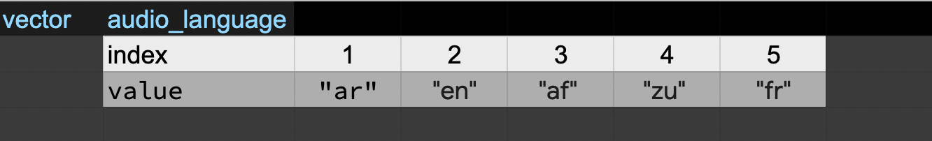
default_l_audio_language <- c("en", "af", "zu")
default_l_audio_language <- c(default_l_audio_language, "fr") # add to the end of the vector
default_l_audio_language <- c("ar", default_l_audio_language) # add to the beginning of the vector
default_l_audio_language

OUTPUT

[1] "ar" "en" "af" "zu" "fr"

In the first line, we take the original vector default_l_audio_language, add the value "fr" to the end of it, and save the result back into default_l_audio_language. Then we add the value "ar" to the beginning, again saving the result back into default_l_audio_language.

We can do this over and over again to grow a vector, or assemble a dataset. As we program, this may be useful to add results that we are collecting or calculating.

An atomic vector is the simplest R data type and is a linear vector of a single type. Above, we saw 2 of the 6 main atomic vector types that R uses: "character" and "numeric" (or "double"). These are the basic building blocks that all R objects are built from. The other 4 atomic vector types are:

• "logical" for TRUE and FALSE (the boolean data type)
• "integer" for integer numbers (e.g., 2L, the L indicates to R that it’s an integer)
• "complex" to represent complex numbers with real and imaginary parts (e.g., 1 + 4i) and that’s all we’re going to say about them
• "raw" for bitstreams that we won’t discuss further

You can check the type of your vector using the typeof() function and inputting your vector as the argument.

Vectors are one of the many data structures that R uses. Other important ones are lists (list), matrices (matrix), data frames (data.frame), factors (factor) and arrays (array).

Exercise

We’ve seen that atomic vectors can be of type character, numeric (or double), integer, and logical. But what happens if we try to mix these types in a single vector?

Show me the solution

R implicitly converts them to all be the same type.

Exercise (continued)

What will happen in each of these examples? (hint: use class() to check the data type of your objects):

R

num_char <- c(1, 2, 3, "a")
num_logical <- c(1, 2, 3, TRUE)
char_logical <- c("a", "b", "c", TRUE)
tricky <- c(1, 2, 3, "4")

Why do you think it happens?

Show me the solution

Vectors can be of only one data type. R tries to convert (coerce) the content of this vector to find a “common denominator” that doesn’t lose any information.

Exercise (continued)

How many values in combined_logical are "TRUE" (as a character) in the following example:

R

num_logical <- c(1, 2, 3, TRUE)
char_logical <- c("a", "b", "c", TRUE)
combined_logical <- c(num_logical, char_logical)

Show me the solution

Only one. There is no memory of past data types, and the coercion happens the first time the vector is evaluated. Therefore, the TRUE in num_logical gets converted into a 1 before it gets converted into "1" in combined_logical.

Exercise (continued)

You’ve probably noticed that objects of different types get converted into a single, shared type within a vector. In R, we call converting objects from one class into another class coercion. These conversions happen according to a hierarchy, whereby some types get preferentially coerced into other types. Can you draw a diagram that represents the hierarchy of how these data types are coerced?

Subsetting vectors

---

Subsetting (sometimes referred to as extracting or indexing) involves accessing out one or more values based on their numeric placement or “index” within a vector. If we want to subset one or several values from a vector, we must provide one index or several indices in square brackets. For instance:

R

audio_language <- c("en", "af", "zu")
audio_language[2]

OUTPUT

[1] "af"

R

audio_language[c(3, 2)]

OUTPUT

[1] "zu" "af"

We can also repeat the indices to create an object with more elements than the original one:

R

extra_audio_language <- audio_language[c(3,2,2,1,3,2)]
extra_audio_language

OUTPUT

[1] "zu" "af" "af" "en" "zu" "af"

R indices start at 1. Programming languages like Fortran, MATLAB, Julia, and R start counting at 1, because that’s what human beings typically do. Languages in the C family (including C++, Java, Perl, and Python) count from 0 because that’s simpler for computers to do.

Conditional subsetting

Another common way of subsetting is by using a logical vector. TRUE will select the element with the same index, while FALSE will not:

R

view_count <- c(120987, 789, 1, 2)
view_count[c(TRUE, FALSE, TRUE, FALSE)]

OUTPUT

[1] 120987      1

Typically, these logical vectors are not typed by hand, but are the output of other functions or logical tests. For instance, if you wanted to select only the values above 5:

R

view_count > 5    # will return logicals with TRUE for the indices that meet the condition

OUTPUT

[1]  TRUE  TRUE FALSE FALSE

R

## so we can use this to select only the values above 5
view_count[view_count > 5]

OUTPUT

[1] 120987    789

You can combine multiple tests using

-& (both conditions are true, AND) or - | (at least one of the conditions is true, OR)

R

view_count[view_count >= 10 | view_count <= 1000]

OUTPUT

[1] 120987    789      1      2

R

view_count[view_count >= 10 & view_count <= 10000]

OUTPUT

[1] 789

Here, < stands for “less than”, > for “greater than”, >= for “greater than or equal to”, and == for “equal to”. The double equal sign == is a test for numerical equality between the left and right hand sides, and should not be confused with the single = sign, which performs variable assignment (similar to <-).

A common task is to search for certain strings in a vector. One could use the “or” operator | to test for equality to multiple values, but this can quickly become tedious.

R

audio_language <- c("ar", "en", "af","zu","fr")
audio_language[audio_language == "zu" | audio_language == "af"] # returns both zu and af

OUTPUT

[1] "af" "zu"

The function %in% allows you to test if any of the elements of a search vector (on the left hand side) are found in the target vector (on the right hand side):

R

audio_language %in% c("en", "fr")

OUTPUT

[1] FALSE  TRUE FALSE FALSE  TRUE

Note that the output is the same length as the search vector on the left hand side, because %in% checks whether each element of the search vector is found somewhere in the target vector. Thus, you can use %in% to select the elements in the search vector that appear in your target vector:

R

audio_language %in% c("en", "af", "xh", "zu","fr","ar")

OUTPUT

[1] TRUE TRUE TRUE TRUE TRUE

R

audio_language[audio_language %in% c("en", "af", "xh", "zu", "fr", "ar")]

OUTPUT

[1] "ar" "en" "af" "zu" "fr"

R

audio_language[audio_language %in% c("en", "fr")]

OUTPUT

[1] "en" "fr"

Missing data

---

As R was designed to analyze datasets, it includes the concept of missing data (which is uncommon in other programming languages). Missing data are represented in vectors as NA.

When doing operations on numbers, most functions will return NA if the data you are working with include missing values. This feature makes it harder to overlook the cases where you are dealing with missing data. You can add the argument na.rm=TRUE to calculate the result while ignoring the missing values.

R

comment_count <- c(2, 1, 1, NA, 7)
mean(comment_count)

OUTPUT

[1] NA

R

max(comment_count)

OUTPUT

[1] NA

R

mean(comment_count, na.rm = TRUE)

OUTPUT

[1] 2.75

R

max(comment_count, na.rm = TRUE)

OUTPUT

[1] 7

If your data include missing values, you may want to become familiar with the functions is.na(), na.omit(), and complete.cases(). See below for examples.

R

## Extract those elements which are not missing values.
## The ! character is also called the NOT operator
comment_count[!is.na(comment_count)]

OUTPUT

[1] 2 1 1 7

R

## Count the number of missing values.
## The output of is.na() is a logical vector (TRUE/FALSE equivalent to 1/0) so the sum() function here is effectively counting
sum(is.na(comment_count))

OUTPUT

[1] 1

R

## Returns the object with incomplete cases removed. The returned object is an atomic vector of type `"numeric"` (or `"double"`).
na.omit(comment_count)

OUTPUT

[1] 2 1 1 7
attr(,"na.action")
[1] 4
attr(,"class")
[1] "omit"

R

## Extract those elements which are complete cases. The returned object is an atomic vector of type `"numeric"` (or `"double"`).
comment_count[complete.cases(comment_count)]

OUTPUT

[1] 2 1 1 7

Recall that you can use the typeof() function to find the type of your atomic vector.

Exercise

1. Using this vector of comments, create a new vector with the NAs removed.

R

comment_count <- c(10000, 2, 19, 1, NA, 3, 1, 3, 2, 1999, 1, 89, 3, 1, NA, 1)

2. Use the function median() to calculate the median of the comment_count vector.

3. Use R to figure out how many videos in the set received more than two comments.

Show me the solution

R

comment_count <- c(10000, 2, 19, 1, NA, 3, 1, 3, 2, 1999, 1, 89, 3, 1, NA, 1)
comments_no_na <- comment_count[!is.na(comment_count)]
# or
comments_no_na <- na.omit(comment_count)
# 2.
median(comment_count, na.rm = TRUE)

OUTPUT

[1] 2.5

R

# 3.
comments_above_2 <- comments_no_na[comments_no_na > 2]
length(comments_above_2)

OUTPUT

[1] 7

Now that we have learned how to write scripts, and the basics of R’s data structures, we are ready to start working with the YouTube dataset we have been using in the other lessons, and learn about data frames.

Key Points

• Access individual values by location using [].
• Access arbitrary sets of data using [c(...)].
• Use logical operations and logical vectors to access subsets of data.