Data Wrangling with tidyr

Overview

Questions

• How can I reformat a data frame to meet my needs?

Objectives

• Describe the concept of a wide and a long table format and for which purpose those formats are useful.
• Describe the roles of variable names and their associated values when a table is reshaped.
• Reshape a dataframe from long to wide format and back with the pivot_wider and pivot_longer commands from the tidyr package.
• Export a dataframe to a csv file.

dplyr pairs nicely with tidyr which enables you to swiftly convert between different data formats (long vs. wide) for plotting and analysis. To learn more about tidyr after the workshop, you may want to check out this handy data tidying with tidyr cheatsheet.

To make sure everyone will use the same dataset for this lesson, we’ll read again the SAFI dataset that we downloaded earlier.

R

library(tidyverse)
library(here)

videos <- read_csv(
  here("data", "youtube-27082024-open-refine-200-na.csv"), 
  na = "na")

R

## inspect the data
videos

OUTPUT

# A tibble: 200 × 32
   position randomise channel_id               channel_title      video_id url
      <dbl>     <dbl> <chr>                    <chr>              <chr>    <chr>
 1      112       409 UCI3RT5PGmdi1KVp9FG_CneA eNCA               iPUAl1j… http…
 2       50       702 UCI3RT5PGmdi1KVp9FG_CneA eNCA               YUmIAd_… http…
 3      149       313 UCMwDXpWEVQVw4ZF7z-E4NoA StellenboschNews … v8XfpOi… http…
 4      167       384 UCsqKkYLOaJ9oBwq9rxFyZMw SOUTH AFRICAN POL… lnLdo2k… http…
 5      195       606 UC5G5Dy8-mmp27jo6Frht7iQ Umgosi Entertainm… XN6toca… http…
 6      213       423 UCC1udUghY9dloGMuvZzZEzA The Tea World      rh2Nz78… http…
 7      145       452 UCaCcVtl9O3h5en4m-_edhZg Celeb LaLa Land    1l5GZ0N… http…
 8      315       276 UCAurTjb6Ewz21vjfTs1wZxw NOSIPHO NZAMA      j4Y022C… http…
 9      190       321 UCBlX1mnsIFZRqsyRNvpW_rA Zandile Mhlambi    gf2YNN6… http…
10      214       762 UClY87IoUANFZtswyC9GeecQ Beauty recipes     AGJmRd4… http…
# ℹ 190 more rows
# ℹ 26 more variables: published_at <dttm>, published_at_sql <chr>, year <dbl>,
#   month <dbl>, day <dbl>, video_title <chr>, video_description <chr>,
#   tags <chr>, video_category_label <chr>, topic_categories <chr>,
#   duration_sec <dbl>, definition <chr>, caption <lgl>,
#   default_language <chr>, default_l_audio_language <chr>,
#   thumbnail_maxres <chr>, licensed_content <dbl>, …

R

## preview the data
# view(videos)

Reshaping with pivot_wider() and pivot_longer()

---

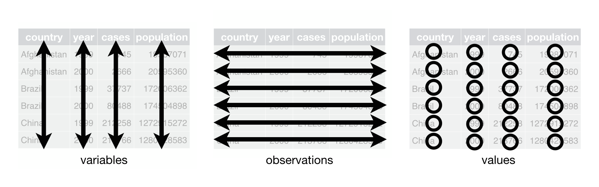
There are essentially three rules that define a “tidy” dataset:

1. Each variable has its own column
2. Each observation has its own row
3. Each value must have its own cell

This graphic visually represents the three rules that define a “tidy” dataset:

R for Data Science, Wickham H and Grolemund G (https://r4ds.had.co.nz/index.html) © Wickham, Grolemund 2017 This image is licenced under Attribution-NonCommercial-NoDerivs 3.0 United States (CC-BY-NC-ND 3.0 US)

In this section we will explore how these rules are linked to the different data formats researchers are often interested in: “wide” and “long”. This tutorial will help you efficiently transform your data shape regardless of original format. First we will explore qualities of the videos data and how they relate to these different types of data formats.

Long and wide data formats

In the videos data, each row contains the values of variables associated with each record collected (each interview in the villages). The video_id identifier is a unique identifier for each YouTube video.

R

videos %>% 
  select(video_id) %>% 
  distinct() %>% 
  count()

OUTPUT

# A tibble: 1 × 1
      n
  <int>
1   200

As seen in the code below, for each time of publication in each channel no video_id`s are the same. Thus, this format is what is called a “long” data format, where each observation occupies only one row in the dataframe.

R

videos %>%
  filter(channel_title == "eNCA") %>%
  select(video_id, channel_title, published_at_sql) %>%
  sample_n(size = 10)

OUTPUT

# A tibble: 10 × 3
   video_id    channel_title published_at_sql
   <chr>       <chr>         <chr>
 1 59uEjm0OlRs eNCA          2020-09-07 8:13:41
 2 vaSOdyC3iNk eNCA          2020-09-04 11:32:18
 3 iPUAl1jywdU eNCA          2020-09-14 16:16:44
 4 -vdIFk95vPk eNCA          2020-09-07 8:23:46
 5 flzoE9zL_KA eNCA          2020-09-07 11:28:32
 6 3EtH4eDceFY eNCA          2020-09-10 9:11:44
 7 3BkmO0M56lA eNCA          2020-09-08 6:54:04
 8 huI9qbGqNhA eNCA          2020-09-07 17:59:13
 9 qvd3C1ZAAmQ eNCA          2020-09-08 16:57:47
10 RGXqGXPQNVE eNCA          2020-09-07 13:18:00

We notice that the layout or format of the videos data is in a format that adheres to rules 1-3, where

• each column is a variable
• each row is an observation
• each value has its own cell

This is called a “long” data format. But, we notice that each column represents a different variable. In the “longest” data format there would only be three columns, one for the id variable, one for the observed variable, and one for the observed value (of that variable). This data format is quite unsightly and difficult to work with, so you will rarely see it in use.

Alternatively, in a “wide” data format we see modifications to rule 1, where each column no longer represents a single variable. Instead, columns can represent different levels/values of a variable. For instance, in some data you encounter the researchers may have chosen for every survey date to be a different column.

These may sound like dramatically different data layouts, but there are some tools that make transitions between these layouts much simpler than you might think! The gif below shows how these two formats relate to each other, and gives you an idea of how we can use R to shift from one format to the other.

Long and wide dataframe layouts mainly affect readability. You may find that visually you may prefer the “wide” format, since you can see more of the data on the screen. However, all of the R functions we have used thus far expect for your data to be in a “long” data format. This is because the long format is more machine readable and is closer to the formatting of databases.

Questions which warrant different data formats

In our dataset of YouTube videos, each row contains the values of variables associated with each record (the unit), values such as the title of the channel which posted the video, the number of views, or the title and description for the video. This format allows for us to make comparisons across individual videos, but what if we wanted to look at differences in videos grouped by different topics or tags associated with the video?

To facilitate this comparison we would need to create a new table where each row (the unit) was comprised of values of variables associated with topics or tags (i.e., the columns topic_categories or tags in the dataset). In practical terms this means the values of the topics in topic_categories (e.g. politics, health, business, society, etc.) would become the names of column variables and the cells would contain values of TRUE or FALSE, for whether the video fitted into that category or not.

Once we we’ve created this new table, we can explore the relationship within and between videos. The key point here is that we are still following a tidy data structure, but we have reshaped the data according to the observations of interest.

Alternatively, consider what we would do if the interview dates were spread across multiple columns, and we were interested in visualizing how the controversy changed over time.

This would require for the interview date to be included in a single column rather than spread across multiple columns. Thus, we would need to transform the column names into values of a single variable.

We can do both of these transformations with two tidyr functions, pivot_wider() and pivot_longer().

Pivoting wider

---

pivot_wider() takes three principal arguments:

1. the data
2. the names_from column variable whose values will become new column names.
3. the values_from column variable whose values will fill the new column variables.

Further arguments include values_fill which, if set, fills in missing values with the value provided.

Let’s use pivot_wider() to transform videos to create new columns for each topic category allocated to a video. There are a couple of new concepts in this transformation, so let’s walk through it line by line. First we create a new object (videos_topics) based on the videos data frame.

R

videos_topics <- videos %>%

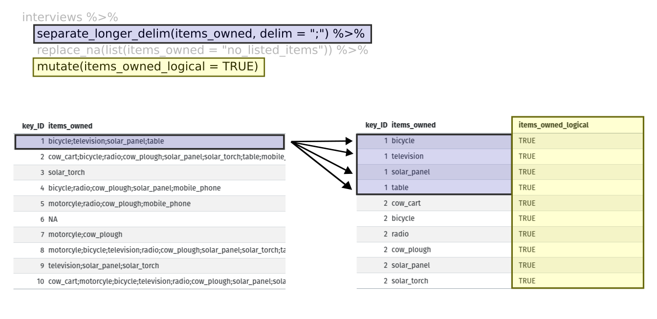
Then we will actually need to make our data frame longer, because we have multiple items in a single cell. We will use a new function, separate_longer_delim(), from the tidyr package to separate the values of topic_categories based on the presence of semi-colons (;). The values of this variable were multiple items separated by semi-colons, so this action creates a row for each item listed in a household’s possession. Thus, we end up with a long format version of the dataset, with multiple rows for each respondent. For example, if a respondent has a television and a solar panel, that respondent will now have two rows, one with “television” and the other with “solar panel” in the topic_categories column.

R

separate_longer_delim(topic_categories, delim = ";") %>%

After this transformation, you may notice that the topic_categories column contains NA values. This is because some of the respondents did not own any of the items that was in the interviewer’s list. We can use the replace_na() function to change these NA values to something more meaningful. The replace_na() function expects for you to give it a list() of columns that you would like to replace the NA values in, and the value that you would like to replace the NAs. This ends up looking like this:

R

replace_na(list(topic_categories = "no_categories")) %>%

Next, we create a new variable named topic_categories_logical, which has one value (TRUE) for every row. This makes sense, since each item in every row was owned by that household. We are constructing this variable so that when we spread the topic_categories across multiple columns, we can fill the values of those columns with logical values describing whether the household did (TRUE) or didn’t (FALSE) own that particular item.

R

mutate(topic_categories_logical = TRUE) %>%

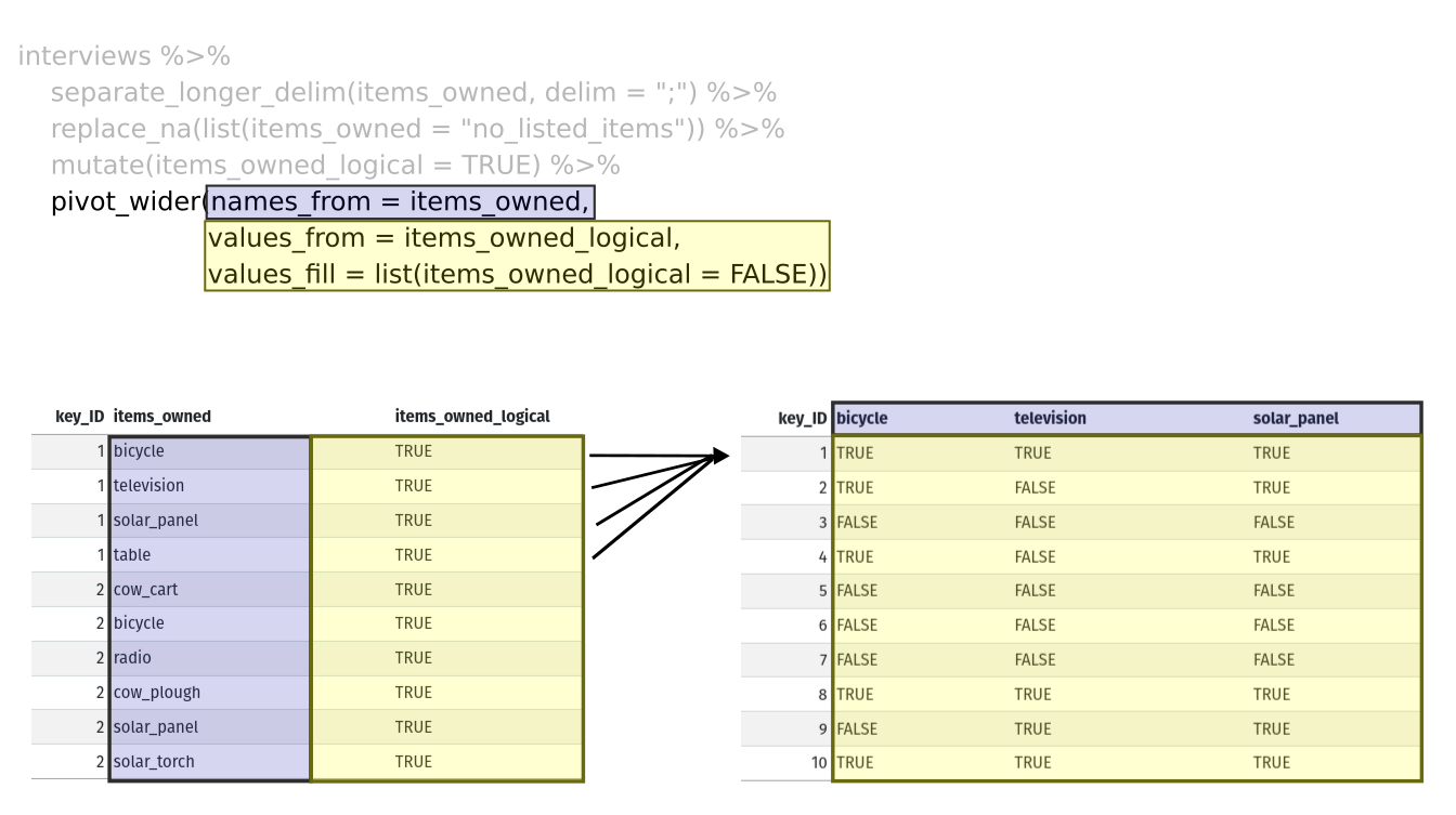
Lastly, we use pivot_wider() to switch from long format to wide format. This creates a new column for each of the unique values in the topic_categories column, and fills those columns with the values of topic_categories_logical. We also declare that for topics that are missing, we want to fill those cells with the value of FALSE instead of NA.

R

pivot_wider(names_from = topic_categories,
            values_from = topic_categories_logical,
            values_fill = list(topic_categories_logical = FALSE))

Combining the above steps, the chunk looks like this:

R

videos_topics <- videos %>%
  separate_longer_delim(topic_categories, delim = ";") %>%
  replace_na(list(topic_categories = "no_topics")) %>%
  mutate(topic_categories_logical = TRUE) %>%
  pivot_wider(names_from = topic_categories,
              values_from = topic_categories_logical,
              values_fill = list(topic_categories_logical = FALSE))
  videos_topics

OUTPUT

# A tibble: 200 × 41
   position randomise channel_id               channel_title      video_id url
      <dbl>     <dbl> <chr>                    <chr>              <chr>    <chr>
 1      112       409 UCI3RT5PGmdi1KVp9FG_CneA eNCA               iPUAl1j… http…
 2       50       702 UCI3RT5PGmdi1KVp9FG_CneA eNCA               YUmIAd_… http…
 3      149       313 UCMwDXpWEVQVw4ZF7z-E4NoA StellenboschNews … v8XfpOi… http…
 4      167       384 UCsqKkYLOaJ9oBwq9rxFyZMw SOUTH AFRICAN POL… lnLdo2k… http…
 5      195       606 UC5G5Dy8-mmp27jo6Frht7iQ Umgosi Entertainm… XN6toca… http…
 6      213       423 UCC1udUghY9dloGMuvZzZEzA The Tea World      rh2Nz78… http…
 7      145       452 UCaCcVtl9O3h5en4m-_edhZg Celeb LaLa Land    1l5GZ0N… http…
 8      315       276 UCAurTjb6Ewz21vjfTs1wZxw NOSIPHO NZAMA      j4Y022C… http…
 9      190       321 UCBlX1mnsIFZRqsyRNvpW_rA Zandile Mhlambi    gf2YNN6… http…
10      214       762 UClY87IoUANFZtswyC9GeecQ Beauty recipes     AGJmRd4… http…
# ℹ 190 more rows
# ℹ 35 more variables: published_at <dttm>, published_at_sql <chr>, year <dbl>,
#   month <dbl>, day <dbl>, video_title <chr>, video_description <chr>,
#   tags <chr>, video_category_label <chr>, duration_sec <dbl>,
#   definition <chr>, caption <lgl>, default_language <chr>,
#   default_l_audio_language <chr>, thumbnail_maxres <chr>,
#   licensed_content <dbl>, location_description <chr>, view_count <dbl>, …

View the videos_topics data frame. It should have 200 rows (the same number of rows you had originally), but extra columns for each item. How many columns were added? Notice that there is no longer a column titled topic_categories. This is because there is a default parameter in pivot_wider() that drops the original column. The values that were in that column have now become columns named politics, health, business, etc. You can use dim(videos) and dim(videos_wide) to see how the number of columns has changed between the two datasets.

This format of the data allows us to do interesting things, like make a table showing the number of videos in each video category on a particular topic:

R

videos_topics %>%
  filter(politics) %>%
  group_by(video_category_label) %>%
  count(politics)

OUTPUT

# A tibble: 4 × 3
# Groups:   video_category_label [4]
  video_category_label politics     n
  <chr>                <lgl>    <int>
1 Comedy               TRUE         1
2 Entertainment        TRUE         5
3 News & Politics      TRUE        24
4 People & Blogs       TRUE        10

Or below we calculate the average number of topics addressed by each channel. This code uses the rowSums() function to count the number of TRUE values in the business to politics columns for each row, hence its name. Note that we replaced NA values with the value no_topics, so we must exclude this value in the aggregation. We then group the data by channel and calculate the mean number of topics, so each average is grouped by channel.

R

videos_topics %>%
    select(-no_topics) %>% 
    mutate(number_topics = rowSums(select(., business:politics))) %>%
    group_by(channel_title) %>%
    summarize(mean_topics = mean(number_topics))

OUTPUT

# A tibble: 119 × 2
   channel_title                 mean_topics
   <chr>                               <dbl>
 1 2nacheki                              1.5
 2 Absolute Controversy                  1
 3 African Diaspora News Channel         1
 4 Al Jazeera English                    2
 5 Ayanda Mafuyeka                       1
 6 Azana Jezile                          1
 7 BANELE NOCUZE                         1
 8 Banetsi Tshetlo                       1
 9 Beauty recipes                        2
10 Blackish Blue TV                      2
# ℹ 109 more rows

Pivoting longer

---

The opposing situation could occur if we had been provided with data in the form of videos_wide, where the items owned are column names, but we wish to treat them as values of an topic_categories variable instead.

In this situation we are gathering these columns turning them into a pair of new variables. One variable includes the column names as values, and the other variable contains the values in each cell previously associated with the column names. We will do this in two steps to make this process a bit clearer.

pivot_longer() takes four principal arguments:

1. the data
2. cols are the names of the columns we use to fill the new values variable (or to drop).
3. the names_to column variable we wish to create from the cols provided.
4. the values_to column variable we wish to create and fill with values associated with the cols provided.

R

videos_long <- videos_topics %>%
  pivot_longer(cols = business:politics,
               names_to = "topic_categories",
               values_to = "topic_categories_logical")

View both videos_long and videos_topics and compare their structure.

Exercise

We created some summary tables on videos_topics using count and summarise. We can create the same tables on videos_long, but this will require a different process.

1. Make a table showing showing the number of videos from each channel categorised as a particular topic, and include all items. The difference between this format and the wide format is that you can now count all the topics using the topic_categories variable.

Show me the solution

R

videos_long %>%
  filter(topic_categories_logical) %>% 
  group_by(channel_title) %>% 
  count(topic_categories, sort=TRUE)

OUTPUT

# A tibble: 171 × 3
# Groups:   channel_title [114]
   channel_title   topic_categories       n
   <chr>           <chr>              <int>
 1 SABC News       society               22
 2 eNCA            society               20
 3 eNCA            television_program    19
 4 SABC News       television_program    14
 5 Newzroom Afrika society               13
 6 Newzroom Afrika television_program    11
 7 SABC News       health                10
 8 eNCA            health                 8
 9 eNCA            politics               6
10 Newzroom Afrika politics               5
# ℹ 161 more rows

Exercise (continued)

2. Calculate the average number of items from the list owned by respondents in each village. If you remove rows where topic_categories_logical is FALSE you will have a data frame where the number of rows per household is equal to the number of items owned. You can use that to calculate the mean number of items per village.

Remember, you need to make sure we don’t count no_listed_items, since this is not an actual item, but rather the absence thereof.

Show me the solution

R

videos_long %>% 
  filter(topic_categories_logical,
         topic_categories != "no_topics") %>% 
  # to keep information per video, we count video_id
  count(video_id, channel_title) %>% # we want to also keep the channel variable
  group_by(channel_title) %>% 
  summarise(mean_topics = mean(n))

OUTPUT

# A tibble: 114 × 2
   channel_title                 mean_topics
   <chr>                               <dbl>
 1 2nacheki                              1.5
 2 Absolute Controversy                  1
 3 African Diaspora News Channel         1
 4 Al Jazeera English                    2
 5 Ayanda Mafuyeka                       2
 6 Azana Jezile                          1
 7 BANELE NOCUZE                         1
 8 Banetsi Tshetlo                       1
 9 Beauty recipes                        2
10 Blackish Blue TV                      2
# ℹ 104 more rows

Applying what we learned to clean our data

---

Now we have simultaneously learned about pivot_longer() and pivot_wider(), and fixed a problem in the way our data is structured. In the spreadsheets lesson, we learned that it’s best practice to have only a single piece of information in each cell of your spreadsheet. In this dataset, we have another column that stores multiple values in a single cell. Some of the cells in the tags column contain multiple months which, as before, are separated by semi-colons (;).

To create a data frame where each of the columns contain only one value per cell, we can repeat the steps we applied to topic_categories and apply them to tags. Since we will be using this data frame for the next episode, we will call it videos_plotting.

R

videos_plotting <- videos %>%
  ## pivot wider by topic_categories
  separate_longer_delim(topic_categories, delim = ";") %>%
  ## if there were no topics listed, changing NA to no_listed_items
  replace_na(list(topic_categories = "no_topics")) %>%
  mutate(topic_categories_logical = TRUE) %>%
  pivot_wider(names_from = topic_categories,
              values_from = topic_categories_logical,
              values_fill = list(topic_categories_logical = FALSE)) #%>%
  ## pivot wider by tags
  #separate_longer_delim(tags, delim = ";") %>%
  #mutate(tags_logical = TRUE) %>%
  #pivot_wider(names_from = tags,
  #           values_from = tags_logical
  #          values_fill = list(tags_logical = FALSE)) %>%
  ## add some summary columns
  #mutate(number_tags = rowSums(select(., Jan:May))) %>% #replace with start and end tags
  #mutate(number_topics = rowSums(select(., business:politics)))

  videos_plotting

OUTPUT

# A tibble: 200 × 41
   position randomise channel_id               channel_title      video_id url
      <dbl>     <dbl> <chr>                    <chr>              <chr>    <chr>
 1      112       409 UCI3RT5PGmdi1KVp9FG_CneA eNCA               iPUAl1j… http…
 2       50       702 UCI3RT5PGmdi1KVp9FG_CneA eNCA               YUmIAd_… http…
 3      149       313 UCMwDXpWEVQVw4ZF7z-E4NoA StellenboschNews … v8XfpOi… http…
 4      167       384 UCsqKkYLOaJ9oBwq9rxFyZMw SOUTH AFRICAN POL… lnLdo2k… http…
 5      195       606 UC5G5Dy8-mmp27jo6Frht7iQ Umgosi Entertainm… XN6toca… http…
 6      213       423 UCC1udUghY9dloGMuvZzZEzA The Tea World      rh2Nz78… http…
 7      145       452 UCaCcVtl9O3h5en4m-_edhZg Celeb LaLa Land    1l5GZ0N… http…
 8      315       276 UCAurTjb6Ewz21vjfTs1wZxw NOSIPHO NZAMA      j4Y022C… http…
 9      190       321 UCBlX1mnsIFZRqsyRNvpW_rA Zandile Mhlambi    gf2YNN6… http…
10      214       762 UClY87IoUANFZtswyC9GeecQ Beauty recipes     AGJmRd4… http…
# ℹ 190 more rows
# ℹ 35 more variables: published_at <dttm>, published_at_sql <chr>, year <dbl>,
#   month <dbl>, day <dbl>, video_title <chr>, video_description <chr>,
#   tags <chr>, video_category_label <chr>, duration_sec <dbl>,
#   definition <chr>, caption <lgl>, default_language <chr>,
#   default_l_audio_language <chr>, thumbnail_maxres <chr>,
#   licensed_content <dbl>, location_description <chr>, view_count <dbl>, …

Exporting data

---

Now that you have learned how to use dplyr and tidyr to wrangle your raw data, you may want to export these new datasets to share them with your collaborators or for archival purposes.

Similar to the read_csv() function used for reading CSV files into R, there is a write_csv() function that generates CSV files from data frames.

Before using write_csv(), we are going to create a new folder, data_output, in our working directory that will store this generated dataset. We don’t want to write generated datasets in the same directory as our raw data. It’s good practice to keep them separate. The data folder should only contain the raw, unaltered data, and should be left alone to make sure we don’t delete or modify it. In contrast, our script will generate the contents of the data_output directory, so even if the files it contains are deleted, we can always re-generate them.

In preparation for our next lesson on plotting, we created a version of the dataset where each of the columns includes only one data value. Now we can save this data frame to our data_output directory.

R

write_csv (videos_plotting, file = "data_output/videos_plotting.csv")

Key Points

• Use the tidyr package to change the layout of data frames.
• Use pivot_wider() to go from long to wide format.
• Use pivot_longer() to go from wide to long format.